Math 118: Compendium
This document contains all of the definitions, facts, and theorems you need to memorize for weekly assessments.
Quick metric for success: During the quiz, if I were to walk up to you and ask you any definition from this list, you will be able to recall it by heart.
Week 1
1.0: The Beginning
Terms are entities separated by subtraction and addition.
Factors are entities separated by multiplication.
Global context refers to the context of the entire expression.
Local context refers to a context smaller than the entire expression.
1.1: Real Numbers
- $\dfrac{a}{b}\cdot \dfrac{c}{d} = \dfrac{ac}{bd}$
- $\dfrac{a}{b}\div \dfrac{c}{d} = \dfrac{a}{b}\cdot \dfrac{d}{c}$
- $\dfrac{a}{c} \pm \dfrac{b}{c} = \dfrac{a \pm b}{c}$
- $\dfrac{a}{b} + \dfrac{c}{d}\qquad $ Find the LCD, then use Fraction Law 3.
- $\dfrac{ac}{bc} = \dfrac{a}{b}$
- Commutative Properties
- $a + b = b + a$
- $ab = ba$
- Associative Properties
- $(a + b) + c = a + (b + c)$
- $(ab)c = a(bc)$
Tip: in English, the commutative/associative properties only interact within the same context level (e.g. only in L3)!
- Distributive Property
- $a(b + c) = ab + ac$
- $(b+c)a = ab + ac$
Tip: in English, the distributive law describes how terms and factors interact.
This is the only way they can interact; anything else is false.
- $(-1)a = -a$
- $-(-a) = a$
- $(-a)(-b) = ab$
- $-(a+b) = -a-b$
1.2: Exponents and Radicals
- $a^ma^n = a^{m+n}$
- $\dfrac{a^m}{a^n} = a^{m-n}$
- $(a^m)^n = a^{mn}$
- $(ab)^n = a^nb^n$
- $\left(\dfrac{a}{b}\right)^n = \dfrac{a^n}{b^n}$
- $\left(\dfrac{a}{b}\right)^{-n} = \dfrac{b^n}{a^n}$
- $\dfrac{a^{-n}}{b^{-m}} = \dfrac{b^m}{a^n}$
Week 2
1.3: Expanding and Factoring
Like terms are terms with the same factors except for the numerical factor (called the coefficient).
- $(A + B)(A - B) = A^2 - B^2$
- $(A + B)^2 = A^2 + 2AB + B^2$
- $(A - B)^2 = A^2 - 2AB + B^2$
Memorize and be able to use the four methods of factoring.
- $A^2 - B^2 = (A-B)(A+B)$
- $A^2 + 2AB + B^2 = (A+B)^2$
- $A^2 - 2AB + B^2 = (A-B)^2$
| Number of Terms | Factoring Methods to Try (in order) |
|---|---|
| 2 terms | GCF, $A^2 - B^2$ |
| 3 terms | GCF, $ax^2 + bx + c, A^2 + 2AB + B^2, A^2 - 2AB + B^2$ |
| 4 terms | GCF, grouping |
| $\geq$ 5 terms | GCF |
Week 3
1.4: Dealing with Rational Expressions
We wrote this down already, but it's worth really memorizing it so you know how to manipulate fractions.
-
$\dfrac{a}{b}\cdot \dfrac{c}{d} = \dfrac{ac}{bd}$
Meaning Multiplying fractions requires multiplying the entire global context of the numerators and the entire global context of the denominators. -
$\dfrac{a}{b}\div \dfrac{c}{d} = \dfrac{a}{b}\cdot \dfrac{d}{c}$
Meaning Dividing fractions requires taking the reciprocal of the right fraction, then multiplying. -
$\dfrac{a}{c} + \dfrac{b}{c} = \dfrac{a + b}{c}$
Meaning Adding fractions with the same denominator requires adding the entire global context of the numerators together. - $\dfrac{a}{b} + \dfrac{c}{d}\qquad $ Find the LCD, then use Fraction Law 3.
-
$\dfrac{ac}{bc} = \dfrac{a}{b}$
Meaning Cancelling an entity requires the entity to be a global factor.
1.5: Equations
- Given $A = B$, we also know $A + C = B + C$.
- Given $A = B$, we also know $A\cdot C = B\cdot C$ provided $C \neq 0$.
Week 4
1.6: Complex Numbers
A complex number has the form \[a + bi\] where $a, b$ are real numbers and $i^2 = -1$. Also, $i = \sqrt{-1}$.
$a$ is called the real part, while $b$ is called the imaginary part.
- If $b^2 - 4ac > 0$, there are two distinct (different) real solutions.
- If $b^2 - 4ac = 0$, there is one real solution.
- If $b^2 - 4ac < 0$, there are two distinct complex solutions.
1.8: Inequalities
- If $A \leq B$, then $A \pm C \leq B \pm C$.
English Adding the same number on both sides does not flip the inequality. - If $C > 0$, then given $A \leq B$, we know $A\cdot C \leq B\cdot C$.
English Multiplying a positive number on both sides does not flip the inequality. - If $C < 0$, then:
- Given $A \leq B$, we know $A\cdot C \geq B \cdot C$
- Given $A < B$, we know $A\cdot C > B \cdot C$
English Multiplying a negative number on both sides flips the inequality.
1.9: Coordinate Plane, Graphs of Equations
The coordinate plane describes where a point is in two dimensional space.

The $y$-intercept of a graph is the $y$-coordinate where the graph intersects the $y$-axis.
1.10: Lines

- The vertical line through $(a, b)$ is $x = a$.
- The horizontal line through $(a, b)$ is $y = b$.
2.1: Functions

The domain of a function is the set of all possible inputs, when evaluated, gives you a real number.
Week 5
2.2: Graphs of Functions
A curve in the plane is the graph of a function if no vertical intersects the curve more than once.
2.3: Using the Graph
Imagine the points drop straight down by gravity:

The solutions to the equation $f(x) = g(x)$ are the $x$-values where the graphs intersect.
The solutions to the inequality $f(x) < g(x)$ are the $x$-values where the graph of $f(x)$ is under $g(x)$.
$f$ is increasing on an interval $I$ if $f(x_1) < f(x_2)$ whenever $x_1 < x_2$ in $I$.
$f$ is decreasing on an interval $I$ if $f(x_1) > f(x_2)$ whenever $x_1 < x_2$ in $I$.
The number $f(a)$ is a local maximum value of $f$ if $f(a) \geq f(x)$ when $x$ is near $a$.
The number $f(a)$ is a local minimum value of $f$ if $f(a) \leq f(x)$ when $x$ is near $a$.
2.4: Average Rate of Change of a Function
The average rate of change (ARoC) of $y = f(x)$ on the interval $(a, b)$ is \[\text{ARoC} = \dfrac{\text{change in } y}{\text{change in } x} = \dfrac{f(b) - f(a)}{b - a}\] The ARoC is the slope of the line through $(a, f(a))$ and $(b, f(b))$.
2.6: Transformations of Functions
Parent functions are functions that have different shapes, based on their formula. Memorize the following.


 $\large f(x) = \sqrt{x}$
$\large f(x) = \lvert x \rvert$
$\large f(x) = \sqrt{x}$
$\large f(x) = \lvert x \rvert$

 To graph $y = f(x) - c$, shift $f(x)$ downwards $c$ units.

 To graph $y = f(x + c)$, shift $f(x)$ left $c$ units.

 To graph $y = f(-x)$, reflect $f(x)$ around the $y$-axis.
To graph $y = c\cdot f(x)$:


To graph $y = c\cdot f(x)$:
If $0 < c < 1$, shrink $f(x)$ vertically by a factor of $c$.
To graph $y = f(c\cdot x)$:


To graph $y = f(c\cdot x)$:
If $0 < c < 1$, stretch $f(x)$ horizontally by a factor of $\frac{1}{c}$.
Week 6
2.7: New Functions From Old
$+, -, \times, \div$ functions together is simple: just substitute. But...
Given two functions $f$ and $g$, the composite function $f \circ g$ is defined by \[(f\circ g)(x) = f(g(x))\]
2.8: One-to-One Functions and Inverses
In other words, if $x_1\neq x_2$, then it is always the case that $f(x_1) \neq f(x_2)$.
A function is one-to-one if and only if no horizontal line intersects the graph of $f(x)$ more than once.
The codomain of a function $f$ is the set of all possible outputs when $f$ is evaluated on the domain.
Let $f$ be a one-to-one function with domain $A$, codomain $B$. Then the inverse function, denoted $f^{-1}$, has domain $B$ and codomain $A$ and is defined by \[f^{-1}(y) = x \text{ if and only if } f(x) = y\]
Let $f$ be a one-to-one function with domain $A$ and codomain $B$. The inverse function $f^{-1}$ satisfies the following properties \begin{align} f^{-1}(f(x))=x \qquad &\text{ for every } x \text{ in } A\\ f(f^{-1}(x))=x \qquad &\text{ for every } x \text{ in } B \end{align}
- Check $f$ is an one-to-one function. If so, proceed. If not, $f$ does not have an inverse.
- Write $y = f(x)$. If there is a domain restriction, convert the domain restriction into a codomain restriction.
- Solve this equation for $x$ in terms of $y$. Meaning, isolate $x$.
- Interchange $x$ and $y$, including the codomain restriction into a domain restriction if there was one. The resulting equation is $y = f^{-1}(x)$.
3.1: Quadratic Functions
A quadratic function is a polynomial function of degree 2, with form \[f(x) = ax^2 + bx + c \qquad a\neq 0\]
A quadratic function $f(x) = ax^2 + bx + c$ can be expressed in the standard form \[f(x) = a(x - h)^2 + k\] by completing the square.
The vertex of the parabola is $(h, k)$.
Week 7
3.2: Polynomial Functions and Their Graphs
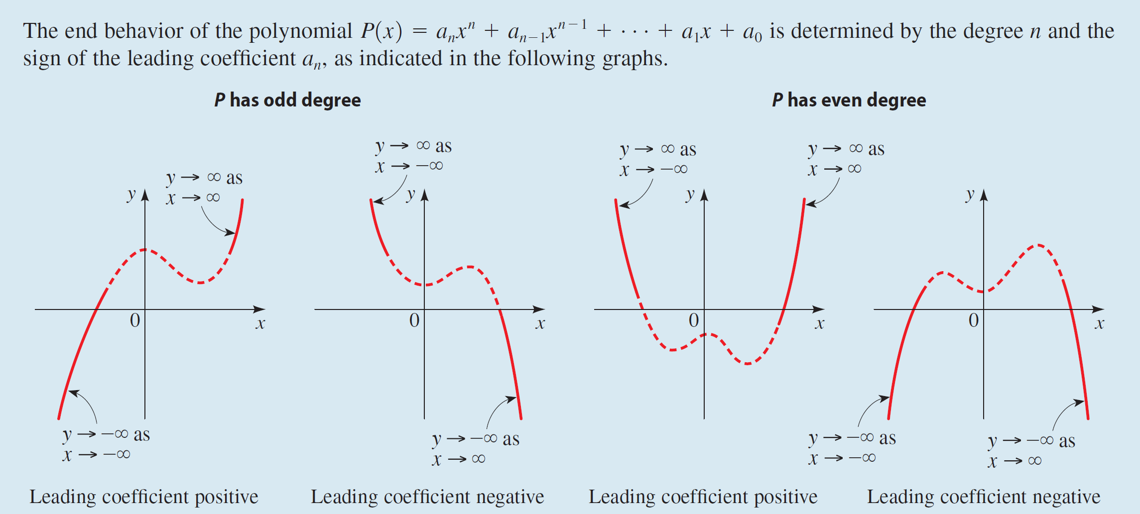
A polynomial function of degree $n$ is a function of the form \[P(x) = a_nx^n + a_{n-1}x^{n-1} + \cdots + a_1x + a_0 \qquad a_n \neq 0\] where $n$ is an integer.
- $a_n, a_{n-1}, \dots, a_1, a_0$ are called the coefficients.
- $a_0$ is called the constant coefficient or constant term.
- $a_n$ is called the leading coefficient.
- $a_nx^n$ is called the leading term.
Monomials $P(x) = x^n$ have the following graphs:


 $n$ is even
$n$ is odd
$n$ is even
$n$ is odd
A graph is continuous if you can draw it without lifting your pencil.
The end behavior of a polynomial depends on the degree $n$ and the leading coefficient $a_n$:
Suppose $P$ is a polynomial and $c$ is a real number. Then the following are equivalent:
- $c$ is a zero of $P$.
- $c$ is a $x$-intercept of the graph of $P$.
- $x = c$ is a solution of the equation $P(x) = 0$. Meaning, $P(c) = 0$.
- $(x - c)$ is a factor of $P(x)$.
$c$ is a zero of multiplicity $m$ if $(x - c)^m$ appears in the factorization of $P$.
If $c$ is a zero of multiplicity $m$, then the graph shape near $c$ corresponds is as follows:
 or
or
 $n$ even
 or
or

$n \neq 1$
or
$n$ even
or
Week 8
3.3: Real Zeros of Polynomials
$P(x)$ and $D(x)$ are polynomials, with $D(x) \neq 0$. Then there exist unique polynomials $Q(x)$ and $R(x)$, where the degree of $R(x)$ is 0 or less than the degree of $P(x)$ where: \[\dfrac{P(x)}{D(x)} = Q(x) + \dfrac{R(x)}{D(x)} \qquad \text{ or } \qquad P(x) = D(x)\cdot Q(x) + R(x)\]
- $P(x)$ is the dividend (what you are dividing)
- $D(x)$ is the divisor (what you are dividing by)
- $Q(x)$ is the quotient
- $R(x)$ is the remainder.
If $P(x)$ is divided by $x - c$, then the remainder is $P(c)$.
$c$ is a zero of $P$ if and only if $(x-c)$ is a factor of $P(x)$.
A complete factorization of a polynomial $P(x)$ over $\mathbb{R}$ is one where the resultant factors only have real coefficients.
For each zero $c$:
- Setup:Convert into a factor $(x - c)$.
- Divide: Use the division algorithm to divide $P(x) = (x - c)Q(x)$.
- Multiplicity: Check if $c$ is a zero of $Q(x)$. If so, repeat and keep dividing $Q(x)$ until $c$ is no longer a zero. Move on to the next zero.
Do not factor irreducibles, leave them alone.
An irreducible polynomial is a quadratic polynomial with no real zeros.
Suppose $P(x)$ is a polynomial with real coefficients. A complete factorization of $P(x)$ over $\mathbb{R}$ will break down into linear (degree 1) factors and irreducible quadratics.
There are three possibilities: \begin{align} P(x) &= (\text{linear factors}) \\P(x) &= (\text{linear factors}) \cdot (\text{irreducible factors}) \\P(x) &= (\text{irreducible factors}) \end{align}3.5: Complex Zeros
Every polynomial \[P(x) = a_nx^n + a_{n-1}x^{n-1} + \cdots + a_1x + a_0 \qquad a_n \neq 0\] with complex coefficients has at least one complex zero.
Suppose $P(x)$ is a degree $n$ polynomial with complex coefficients. Then:
- there exists complex numbers $a, c_1, c_2, \dots, c_n$ where \[P(x) = a(x-c_1)(x-c_2)\cdots(x-c_{n-1})(x-c_{n})\] and
- $P(x)$ has exactly $n$ zeros, provided a zero of multiplicity $k$ is counted $k$ times.
To find a complete factorization of $P(x)$ over $\mathbb{C}$, take the complete factorization over $\mathbb{R}$ and factor the irreducibles into linear factors.
The complex conjugate of $a + bi$ is $a - bi$.
If $P(x)$ has real coefficients and $a + bi$ is a zero, then $a - bi$ must also be a zero.
Week 9
3.6: Rational Functions
A rational function has the form \[r(x) = \dfrac{P(x)}{Q(x)}\]where $P$ and $Q$ are polynomials.
(from the left)
 $x\rightarrow a^+$
(from the right)

(from the left)
$x\rightarrow a^+$(from the right)
The line $y = b$ is a horizontal asymptote if $y \rightarrow b$ as $x \rightarrow \pm \infty$.
- To find vertical asymptotes, set denominator $= 0$ and solve for $x$.
- To find horizontal asymptotes, there are three cases, depending on the leading terms:
- If $n < m$, then $y = 0$ is the horizontal asymptote.
- If $n = m$, then $y = \dfrac{a_n}{b_m}$.
- If $n > m$, there are no horizontal asymptotes.
4.1: Exponential Functions
The exponential function with base $a$ has the form \[f(x) = a^x\] where $a > 0$ and $a \neq 1$.


- Domain: $\mathbb{R}$
- Codomain (range): $(0, \infty)$
- Asymptotes: $y = 0$
Interest applied only once against the principal.
The money invested/borrowed initially.
Compound interest is calculated by \[A(t) = P\left(1 + \dfrac{r}{n}\right)^{nt}\] where
- $A(t) = $ amount after $t$ years
- $P = $ principal
- $r = $ interest rate per year
- $n = $ number of times interest is compounded per year
- $t = $ number of years.
The simple interest rate in one year which accounts for compounding.
4.2: The Natural Exponential Function
The number $e$ is defined to be \[\left(1 + \dfrac{1}{n}\right)^n \rightarrow e \quad \text{as} \quad n \rightarrow \infty\]
Exponential function with base $e$: \[f(x) = e^x\]
Continuously compounded interest is calculated by \[A(t) = Pe^{rt}\] where
- $A(t) = $ amount after $t$ years
- $P = $ principal
- $r = $ interest rate per year
- $t = $ number of years.
Suppose $a > 0, a \neq 1$. The logarithmic function with base $a$ is defined by \[\log_a x = y \qquad \text{means} \qquad a^y = x\]
4.3: Logarithmic Functions
- $\log_a 1 = 0$
- $\log_a a = 1$
- $\log_a a^x = x$
- $a^{\log_a x} = x$
Base 10 logarithm, the base is omitted: \[\log x = \log_{10} x\]
Base $e$ logarithm, denoted by $\ln$: \[\ln x = \log_{e} x\]
- $\ln 1 = 0$
- $\ln e = 1$
- $\ln e^x = x$
- $e^{\ln x} = x$
 In general:
- Domain: $(0, \infty)$
- Codomain (range): $\mathbb{R}$
- Asymptotes: $x = 0$
Week 10
4.4: Laws of Logarithms
Let $a > 0, a \neq 1$ and $A,B,C \in \mathbb{R}$ where $A > 0$ and $B > 0$.
- $\log_a(AB) = \log_a A + \log_a B$
- $\log_a\left(\dfrac{A}{B}\right) = \log_a A - \log_a B$
- $\log_a(A^C) = C\cdot\log_a A$
4.5: Exponential and Logarithmic Equations
- Isolate the exponential expression.
- If there are two exponential expressions, put one on each side.
- Take the logarithm of each side. Bring down the exponent with Laws of Logarithms.
- Solve for the variable.
- Isolate the logarithmic expression (combine with Laws of Logarithms if necessary).
- If there are two logarithmic expressions, put one on each side.
- Write the logarithm in exponential form, or exponentiate both sides with the base.
- Solve for the variable.