1.5: The Limit of a Function
Goals:
- Define the limit of a function
- Describe a tool for calculating the limit of a function.
- Understand when a limit exists and what the graph looks like.
- Describe pitfalls with this method.
The Table Method
We start with an example.
I think about it like this: the heights $f(x)$ can be made as close to $L$ as possible when you move $x$ close to $a$ but never $a$ itself.
This results in three possible graphs: 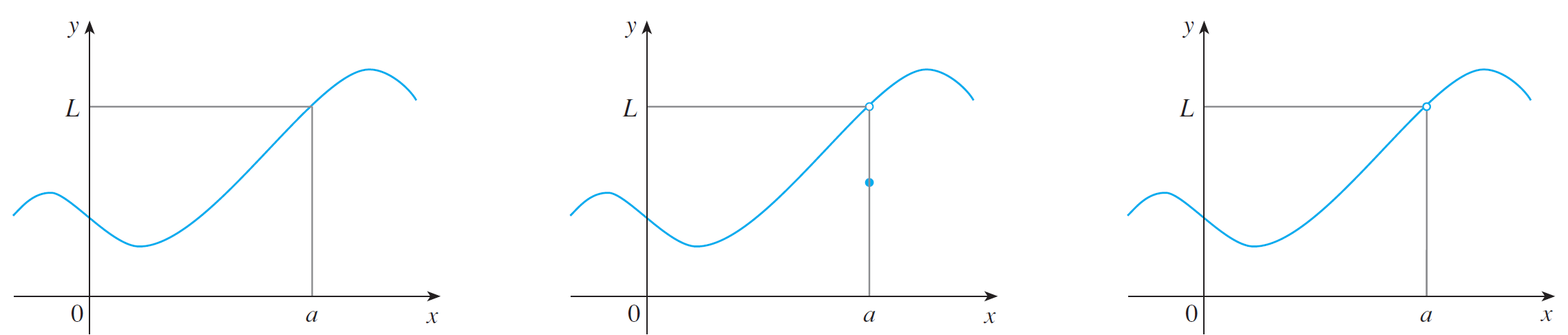
Our first tool for finding limits was described in the first example; it's called the table method. Create two tables that samples $x$ values to the left and right of $a$ but never $a$. Do not plug in $a$!!!!
Then see what the values of $f(x)$ are approaching. If both tables agree then the limit exists.
- $\displaystyle\lim_{x\rightarrow 1} \dfrac{x-1}{x^2 - 1}$
- $\displaystyle\lim_{x\rightarrow 1} g(x)$ where \[g(x) = \begin{cases} \dfrac{x-1}{x^2 - 1} & x \neq 1 \\ 2 & x = 1 \end{cases}\]
- $\displaystyle \lim_{x\rightarrow 0} \dfrac{\sin x}{x}$
- $\displaystyle\lim_{x\rightarrow 0} \left(x^3 + \dfrac{\cos 5x}{10000}\right)$
These examples show that the table method has a big pitfall: potential inaccuracy if you don't pick $x$ close enough to $a$.
One-Sided Limits
The table method requires two tables: one with $x$ values less than $a$, and another with $x$ values greater than $a$.
Here's limit notation for each table:
The function $f$ has the right-hand limit $L$ as $x\rightarrow a$ from the right, written \[\lim_{x\rightarrow a^+} f(x) = L\] if $f(x)$ can be made close to $L$ as we please by taking $x$ sufficiently close to and to the right of $a$.
Similarly, the function $f$ has the left-hand limit $L$ as $x\rightarrow a$ from the left, written \[\lim_{x\rightarrow a^-} f(x) = L\] if $f(x)$ can be made close to $L$ as we please by taking $x$ sufficiently close to and to the left of $a$.
If left-and right-hand limits agree, the limit exists. This is equivalent to both tables agreeing. This idea is summarized as:
This theorem is very important. If left- and right-hand limits disagree, the limit does not exist.
The Graph Method
Limits can also be seen on the graph: look at what the heights of the function are approaching on both sides of $x = a$.
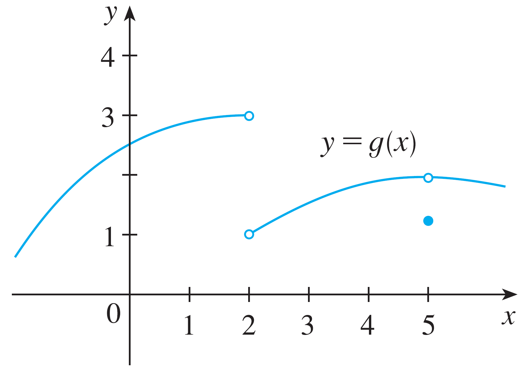 Determine if the following exist. If they do, find the value.
- $\displaystyle\lim_{x\rightarrow2^-} g(x)$
- $\displaystyle\lim_{x\rightarrow2^+} g(x)$
- $\displaystyle\lim_{x\rightarrow2} g(x)$
- $\displaystyle\lim_{x\rightarrow5^-} g(x)$
- $\displaystyle\lim_{x\rightarrow5^+} g(x)$
- $\displaystyle\lim_{x\rightarrow5} g(x)$
- $f(2)$
- $f(5)$
Infinite Limits
The symbol $\infty$ is not a number. Certainly not a real number.
This is why in interval notation you always see $(-\infty, 3)$ or $(0, \infty)$, but never $(0, \infty]$.
Mathematicians use the symbol $\infty$ to represent the idea that a quantity grows forever.
If $\lim_{x\rightarrow a}f(x) = -\infty$, then $f(x)$ is decreasing without bound.
These conditions are equivalent to the existence of a vertical asymptote. See pictures in class.
The definition also applies to left- and right-hand limits, i.e. $\lim_{x\rightarrow a^-} f(x) = \infty$ means the heights of the graph are growing without bound as $x$ approaches $a$ from the left.
In summary, we know two ways to find limits:
- Use the table technique, observe what $f(x)$ is approaching
- Use the graph, observe what the heights $f(x)$ seem to be approaching.